Modeling a Thrust Vector Control Rocket in Python
Rocketry has always been a fascinating topic for me and I’d love to get into model rocketry because it seems so interesting. Unfortunately, due to where I live, I can’t really get into it due to lack of materials, cost, and local laws. So what’s a guy to do when he wants to get into rocketry but can’t physically do it? He goes the virtual simulation route.
I’ll be building a simulation for a simple thrust vector control (TVC) rocket. This rocket will be modeled pretty accurately to life, it won’t be 100% realistic since it’s just a simulation, but it will be mostly correct. I’ll be documenting everything from start to finish so that anyone who wants to can follow along.
Note: We won’t be simulating anything like wind speed or air resistances because that’s a little too complex for the scope of this project. We also won’t be going into any PID or any control stuff. I might add these extra factors and implement some controls into this simulation in the future though.
Measuring the actual rocket
A really important measurement that we need in order to make our simulation is the mass moment of inertia. Mass moment of inertia is about the density across the rocket, this density will come to affect the inertia of the rocket and how “resistant” the rocket will be to change in inertia. The mass distribution also what comes into play when we need to know about the density across the rocket.
I’ll explain briefly about the measurements and how they are taken. If you want a detailed explanation and demonstration, check out this BPS space video. I took the measurements from that video as I don’t have any way to do the measurements on an actual model rocket.
To calculate the mass moment of inertia, we’ll first need the mass (in kg) of the rocket, so just put the rocket on the scale and you’re good to go. Our rocket will have a mass of $0.543kg$
Next, we’ll get the COM-string amount, which will be $0.3m$. And the string length measurement will be $0.65m$. This is the distance of the hang string from the center of mass.
Next, we’ll need to get the moment arm measurement of the rocket. Moment arm is the distance between the attach point of the thrust vector control thruster and the center of mass of the rocket. This measurement will come in handy when we need to calculate for torque. Our moment arm value will be $0.28m$
Next, we’ll need the rotation time between each oscillations, which is basically getting the average time between each oscillation. Our rotation time will be $1.603s$.
Again, this is just a brief explanation on what these measurements are, if you want to see how to actually measure these values, check out the BPS space video above.
To recap, here’s all the measurements and constants that we need to calculate the mass moment of inertia:
- Rocket mass: $m = 0.543kg$
- Gravitational constant: $g = 9.81 m / s^2$
- Rotation time: $R_t = 1.603s$
- Distance between center of mass and string: $d = 0.3m$
- Length of string: $l = 0.65m$
We can then plug these values into the mass moment of inertia equation:
$$ MMOI = \frac{m * g * R_t^2 * d^2}{4 \pi^2 * l} $$
This will give us an MMOI value of $0.048kg \cdot m^2$. With this value and the moment arm value ($0.28m$), we can now build a program to simulate this rocket.
3 Degrees of Freedom
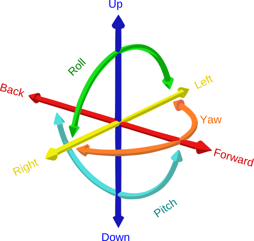
A rocket will usually have 3 degrees of freedom (3DOF), the pitch, the yaw, and the roll. This image (from Wikipedia) will give you a pretty nice visualization on what all these degrees are.
A 3DOF function will help simulate the flight dynamics of the rocket by modeling motions and angles based on the forces and moments applied on it. For this rocket, since we’re doing a 2D simulation, we’ll need to make a 3DOF function to take into account the rotation in the vertical plane about a flat reference frame. We’ll only need to care about the X and Z axes since we’re going 2D so no need to worry about the Y axis.
We’ll need to take in the data of the forces, moments, and mass of the rocket so as to accurately simulate its dynamics. The output will represent the information about the rocket at any time during flight.
Our 3DOF function will need to take in these values:
- The forces on the X and Z axes ($Fx$ and $Fz$)
- The pitching moment ($My$): Represents the torque due to thrust
This 3DOF function will output these values:
- Pitch angle ($\theta$): The angle between the body axis and the reference plane
- Pitch angular rate ($q$): The rate of change of the pitch angle
- Pitch angular acceleration ($dqdt$): The rate of change of the pitch angular rate
- Position ($(x, z)$): Position coordinate of the rocket
- Velocity ($(u, w)$): The velocity in the X and Z axis of the rocket
- Acceleration ($(Ax, Az)$): The acceleration of the rocket
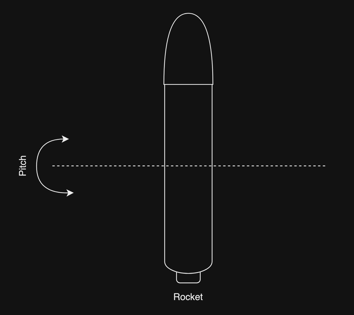
This is the pitch in a rocket:
Implementing the 3DOF function
Before we start coding, we’re going to need to import numpy and matplotlib:
import numpy as np
import matplotlib.pyplot as plt
Let’s start implementing a 3DOF function in Python. This function needs the initial values of the rocket when it has not been launched then it will calculate the state of the rocket as the time increases and we apply thrust to it:
'''
Inputs:
- Fx: Force in the body x-direction (N)
- Fz: Force in the body z-direction (N)
- My: Pitching moment, represents torque (Nm)
- u0: Initial velocity in x (body axis)
- w0: Initial velocity in z (body axis)
- theta0: Initial pitch angle
- q0: Initial pitch rate
- pos0: Starting position [x, z]
- mass: Mass of the rocket
- inertia: Mass moment of inertia
- g: Grativational constant
- dt: Time step
- duration: Duration of simulation
'''
def three_dof_body_axes(Fx, Fz, My, u0=0.0, w0=0.0, theta0=0.0, q0=0.0, pos0=[0.0, 0.0], mass=0, inertia=0.0, g=9.81, dt=0.01, duration=10):
Note that the time step represent a discrete time interval over which calculations will be performed to approximate the continuous changes in the rocket.
All of these values has been set to a default value which we can change later on.
Next, we’ll assign these values to an internal variable so that we can operate on these values:
pos = np.array(pos0, dtype=float) # this ensures that pos0 is a float array
u = u0
w = w0
vel = np.array([u, w]) # assign velocity in X and Z axes to a single variable
theta = theta0
q = q0
While we’re assigning these initial values, we need to also calculate the initial acceleration in the X and Z axes. The calculation is quite easy, we just grab the initial forces in the X and Z axes and divide it by mass (classic $F=ma$), but we need to make sure to subtract the gravitational constant from the acceleration in the Z axis because of gravity. Since our forces in the X and Z axes are stored in arrays (for reasons you’ll see later on), we can just access the initial forces by getting the 0th element:
ax = Fx[0] / mass
az = Fz[0] / mass - g
Then we’ll initialize a list to store the calculated output values. These list will hold the information of the rocket at each time interval during flight.
theta_list = [theta]
q_list = [q]
dqdt_list = [0]
pos_list = [pos.copy()]
velocity_list = [vel.copy()]
acceleration_list = [np.array([ax, az])]
Now, here comes the fun part: the calculation algorithm. Since we’re essentially solving some ordinary differential equations here (The equations describe how a state variable changes over time based on the current state and possible external inputs), we can use Euler’s method to approximate the solutions to these ODEs and iteratively update the state variables in the output lists:
# time integration using Euler's method
for t in np.arange(dt, duration + dt, dt): # start at dt and end at 'duration'
We will run this from for the whole set duration of the simulation, with a time step of $dt$. Since $dt$ was set to $0.01s$, the time step will be quite small, this allows us to collect data of the rocket for each time step for the duration of the simulation, so we’ll be calculating and storing the calculated data every $0.01s$.
Next, we’ll need to calculate the instantaenous acceleration in the X and Z axes based on the forces applied on the rocket on the X and Z axes on a particular time step (by using int(t/dt), we can index the $Fx$ and $Fz$ array at a the current time step $t$):
# calculate accelerations
ax = Fx[int(t/dt)] / mass
az = Fz[int(t/dt)] / mass - g
Next, we’ll calculate the angular acceleration or the rate of change of the pitch angular rate. This is calculated by just dividing the $My$ (the torque) with $inertia$ (the mass moment of inertia). Think of it as dividing the torque with the resistance to the change in inertia. This will give us the rate of change in pitch angular rate for the rocket:
# calculate angular acceleration
dqdt = My[int(t/dt)] / inertia
We’ll also need to calculate the velocities in the X and Z axes along with the pitch angular rate with respect to the previous states:
# calculate velocities and pitch angular rate
u += ax * dt
w += az * dt
q += dqdt * dt
By doing this, our simulation can process how the rocket’s dynamics will evolve over time. We’ll need to do the same thing to get the position, the pitch angle, and the instantenous velocity:
# calculate positions
pos += vel * dt
vel = np.array([u, w])

# calculate angle
theta += q * dt
Ok, that’s all the calculations needed to be done. Now we can store all these values in their respective list:
# store data in list
theta_list.append(theta)
q_list.append(q)
dqdt_list.append(dqdt)
pos_list.append(pos.copy())
velocity_list.append(vel.copy())
acceleration_list.append(np.array([ax, az]))
Finally, to close up this time integration loop, we need a stopping condition for when the rocket hits the Earth plane. We can do this by just checking if the Z position value is less than or equal to 0 and check if the current time in the simulation is larger than 2. We need to set that time condition because we have to allow some time for the rocket to launch from 0:
# stop if the rocket returns to ground level
if pos[1] <= 0 and t > 2:  # allow some time for launch
    break
After the time integration, we can return the state variable lists. And that was our 3DOF function. This is the full code for the function:
def three_dof_body_axes(Fx, Fz, My, u0=0.0, w0=0.0, theta0=0.0, q0=0.0, pos0=[0.0, 0.0], mass=0, inertia=0.0, g=9.81, dt=0.01, duration=10):
    # ensure pos0 is a float array
    pos = np.array(pos0, dtype=float)

    # initial conditions
    u = u0
    w = w0
    theta = theta0
    q = q0
    vel = np.array([u, w])

    # initial acceleration
    ax = Fx[0] / mass
    az = Fz[0] / mass - g

    # lists to store values
    theta_list = [theta]
    q_list = [q]
    dqdt_list = [0]
    pos_list = [pos.copy()]
    velocity_list = [vel.copy()]
    acceleration_list = [np.array([ax, az])]

    # time integration using Euler's method
    for t in np.arange(dt, duration + dt, dt):  # start at dt and end at 'duration'
        # calculate accelerations
        ax = Fx[int(t/dt)] / mass
        az = Fz[int(t/dt)] / mass - g

        # calculate angular acceleration
        dqdt = My[int(t/dt)] / inertia

        # calculate velocities and pitch angular rate
        u += ax * dt
        w += az * dt
        q += dqdt * dt

        # calculate positions
        pos += vel * dt
        vel = np.array([u, w])

        # calculate angle
        theta += q * dt

        # store data in list
        theta_list.append(theta)
        q_list.append(q)
        dqdt_list.append(dqdt)
        pos_list.append(pos.copy())
        velocity_list.append(vel.copy())
        acceleration_list.append(np.array([ax, az]))

        # stop if the rocket returns to ground level
        if pos[1] <= 0 and t > 2:  # allow some time for launch
            break

    return {
        'theta' : np.array(theta_list),
        'q' : np.array(q_list),
        'dqdt' : np.array(dqdt_list),
        'pos' : np.array(pos_list),
        'velocity' : np.array(velocity_list),
        'acceleration' : np.array(acceleration_list)
    }
Thrust profile
A rocket simulation will need some way to generate a thrust profile. The thrust profile is just how much thrust is generated at a certain time step. Our rocket will have a peak thrust of $15N$. Since we’re trying to model our rocket kinda closely to a real model rocket (not absolutely accurate), we’ll need to simulate some of the phases of thrust that will be in a model rocket.
Our rocket will have 4 phases of thrust: Rapid rise, Peak thrust, Decay phase, and Burnout:
- Rapid rise: In this phase, our rocket will quickly ramps up from $0N$ of thrust to $15N$ of thrust. This phase takes up $10%$ of the thrust duration. We can model this after a quadratic rise, this allows our rocket to gradually start and quickly ramp up as time passes.
- Peak thrust: In this phase, our rocket will stay at the peak thrust of $15N$ for the duration of the phase. This phase takes up $20%$ of the thrust duration. Since the thrust value will be constant in this phase, a continous assignment is all that we’ll need for this.
- Decay phase: In this phase, our rocket will gradually reduce the thrust force from $15N$ to $0N$. This phase takes up $70%$ of the thrust duration. We can model this after a linear decay, which is a good approximation for thrust reduction.
- Burnout: In this phase, our rocket’s thrust will be $0N$. This happens after the thrust duration.
Implementing the thrust profile generation function
Let’s start implementing the thrust profile generation in Python. This function will need the simulation duration, the thrust duration, the peak thrust value, and the time step $dt$:
def generate_thrust_profile(duration, thrust_duration, peak_thrust, dt=0.01):
We’ll need to loop through the duration of the simulation and generate a thrust for each time interval. We’ll save the thrust values for each time interval in a thrust profile array:
thrust_profile = []
    for t in np.arange(0, duration + dt, dt):
First, we’ll need to implement the rapid rise phase ($10%$ of total thrust duration):
if t < 0.1 * thrust_duration:
    # ignition and rapid rise (modeled as quadratic rise)
    thrust = peak_thrust * (10 * t / thrust_duration)**2
We’re basically modeling the quadratic rise here. We multiply the t / thrust_duration with 10 to normalize the data to a range of $[0, 1]$, this is basically the percentage time passed. Then we use the power of 2 to make this equation quadratic and the wholething with peak_thrust to get the thrust at $t$. This will give us a slow increase in the beginning and quick ramp up as time increases.
Next, we’ll implement the peak thrust phase ($20%$ of total thrust duration):
elif t < 0.3 * thrust_duration:
    # peak thrust
    thrust = peak_thrust
This will end at around $30%$ of the full thrust duration, since the rapid rise phase already took up $10%$. There’s also no calculation here, we just assign peak_thrust to the thrust variable.
Next, we’ll implement the decay phase ($70%$ of total thrust duration):
elif t < thrust_duration:
    # decay phase (modeled as linear decay)
    thrust = peak_thrust * (1 - (t - 0.3 * thrust_duration) / (0.7 * thrust_duration))
This is modeled after linear decay. Let’s break down each part:
((t - 0.3 * thrust_duration) / (0.7 * thrust_duration))
(t - 0.3 * thrust_duration) gives us the elapsed time since the end of the peak thrust phase, because the peak thrust phase ended at $30%$ of the duration, subtracting that from $t$ will give us the elapsed time.
Then we divide that with (0.7 * thrust_duration) to get the percentage of the elapsed time in the decay phase. Because the decay phase is $70%$ of the duration, and we want to get how long have we been in this decay phase, we divide it with (0.7 * thrust_duration).
(1 - (t - 0.3 * thrust_duration) / (0.7 * thrust_duration))
We will subtract this division from 1 to invert the value because we want the thrust to gradually decay and we want the value of the division to gradually go down.
Finally, we just multiply this with the peak thrust value to get the thrust at a given time interval $t$ during the decay phase.
Next, we’ll implement the burnout phase:
else:
    # burnout
    thrust = 0
Then we just append the thrust value to the thrust profile list we initialized earlier and return it. Here’s the full function:
def generate_thrust_profile(duration, thrust_duration, peak_thrust, dt=0.01):
    thrust_profile = []
    for t in np.arange(0, duration + dt, dt):
        if t < 0.1 * thrust_duration:
            # ignition and rapid rise (modeled as quadratic rise)
            thrust = peak_thrust * (10 * t / thrust_duration)**2
        elif t < 0.3 * thrust_duration:
            # peak thrust
            thrust = peak_thrust
        elif t < thrust_duration:
            # decay phase (modeled as linear decay)
            thrust = peak_thrust * (1 - (t - 0.3 * thrust_duration) / (0.7 * thrust_duration))
        else:
            # burnout
            thrust = 0
        thrust_profile.append(thrust)
    return np.array(thrust_profile)
Let’s test this out by generating a thrust profile and plot it out:
# parameters
peak_thrust = 15 # N
thrust_duration = 4 # s
simulation_duration = 30 # s
dt = 0.01 # time step

# generate thrust profile
thrust_profile = generate_thrust_profile(simulation_duration, thrust_duration, peak_thrust, dt)
time_range = np.arange(0, simulation_duration + dt, dt)

# plot the thrust
plt.figure(figsize=(10, 6))
plt.plot(time_range, thrust_profile, label='Thrust')

# annotate the end of the stages
plt.axvline(x=0.1 * thrust_duration, color='red', linestyle='--', label='End of rapid rise')
plt.axvline(x=0.3 * thrust_duration, color='green', linestyle='--', label='End of peak thrust')
plt.axvline(x=thrust_duration, color='orange', linestyle='--', label='End of decay phase (Burnout)')

plt.xlabel('Time (s)')
plt.ylabel('Thrust (N)')
plt.title('Thrust Profile')
plt.legend()
plt.grid()
plt.show()
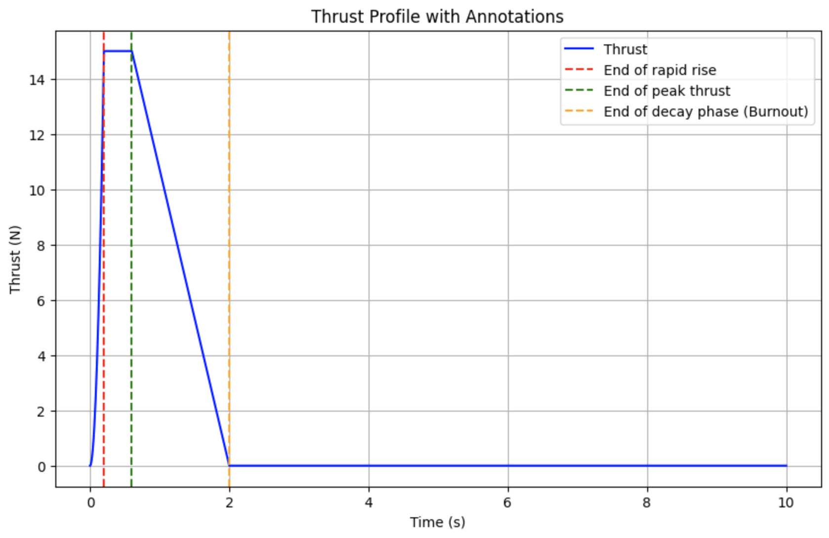
We can see that the rapid rise phase starts out slowly but ramps up very quickly, the peak thrust phase is constant, and the decay phase is linear. So our function is working just fine.
Now that we have our thrust profile generation function, we can finally move on to using it to calculate our rocket’s dynamics and simulate it.
Making the simulation
First, we’ll need to initialize some parameters (using the values we measured before) and setup the initial condition of the rocket. We’ll have a thrust peak value of $15N$ and a thrust duration of 4 seconds. We’ll also set the simulation timeframe to 30 seconds:
# parameters
mass = 0.543 # kg
inertia = 0.048 # kg*m^2
g = 9.81 # m/s^2
peak_thrust = 15 # N
thrust_duration = 4 # s
simulation_duration = 30 # s
dt = 0.01 # time step
moment_arm = 0.28 # meters
gimbal_angle = 0.00 # radian

# initial conditions
u0 = 0.0 # initial velocity in x (body axis)
w0 = 0.0 # initial velocity in z (body axis)
theta0 = 0.0 # initial pitch angle
q0 = 0.0 # initial pitch rate
pos0 = [0.0, 0.0] # initial position [x, z]

# generate thrust profile
thrust_profile = generate_thrust_profile(simulation_duration, thrust_duration, peak_thrust, dt)
Note on the gimbal_angle variable, I initialized this to $0rad$ for now. This will be the angle of the thruster gimbal. We’ll see how changing this value will affect the rocket later on. A gimbal angle of 0 will shoot the rocket straight up.
Next, we’ll need to calculate the force on the X and Z axes along with the torque based on the thrust profile:
# initialize forces and moments
Fx = np.sin(gimbal_angle) * thrust_profile # horizontal thrust
Fz = np.cos(gimbal_angle) * thrust_profile # vertical thrust
My = Fx * moment_arm # pitching moment (torque)
This is some simple trigonometry to calculate the horizontal and vertical thrust of a rocket. Let’s try to visualize this.
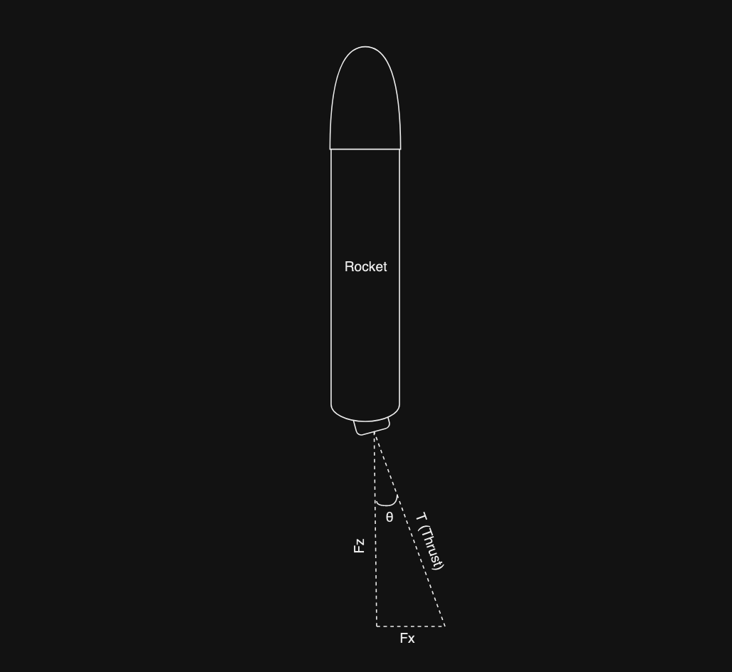
This is how the forces on the X and Z axes can be visualized based on the thrust direction, with $\theta$ being the gimbal angle. With this visualization, we can see how trigonometry can be applied to this problemto calculate the forces on the X and Z axes. By using the soh cah toa rule, we can get these 2 equations:
$$ \sin(\theta) = \frac{F_x}{T}, \ \cos(\theta) = \frac{F_z}{T} $$
Reordering the equations will give us these new equations:
$$ F_x = \sin(\theta) * T, \ F_z = \cos(\theta) * T $$
For the torque, we can just multiply the force applied to the rocket in the X axis with the moment arm because the horizontal thrust will generate a moment around the rocket’s center of mass (this is used to control the pitch, that’s why it’s called pitching moment)
We finally have all the necessary values to plug into our 3DOF function. We’ll also extract the position, velocity and acceleration results into a variable and initialize a time variable for plotting:
results = three_dof_body_axes(Fx, Fz, My, u0, w0, theta0, q0, pos0, mass, inertia, g, dt, simulation_duration)

time = np.arange(0, len(results['pos']) * dt, dt)
pos = results['pos']
velocity = results['velocity']
acceleration = results['acceleration']
Plotting the simulation data with no gimbal angle
Let’s plot all these results out to see how our rocket performed. We’ll plot out the data on the Z axis first:
# plot data (Z axis)
plt.figure(figsize=(12, 8))

plt.subplot(3, 1, 1)
plt.plot(time, pos[:, 1], label='Z Position')
plt.xlabel('Time (s)')
plt.ylabel('Z Position (m)')
plt.title('Z Position Data')
plt.legend()
plt.grid()

plt.subplot(3, 1, 2)
plt.plot(time, velocity[:, 1], label='Z Velocity')
plt.xlabel('Time (s)')
plt.ylabel('Z Velocity (m/s)')
plt.title('Z Velocity Data')
plt.legend()
plt.grid()

plt.subplot(3, 1, 3)
plt.plot(time, acceleration[:, 1], label='Z Acceleration')
plt.xlabel('Time (s)')
plt.ylabel('Z Acceleration (m/s^2)')
plt.title('Z Acceleration Data')
plt.legend()
plt.grid()

plt.tight_layout()
plt.show()
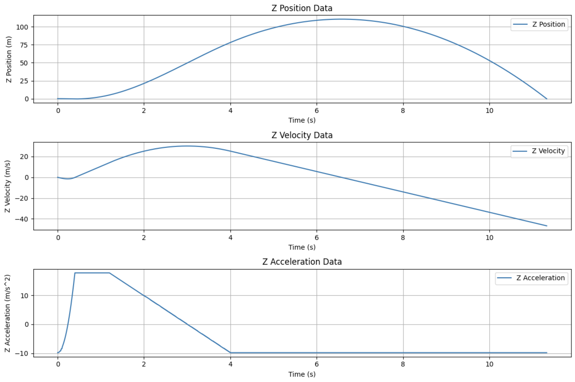
Look at those curves. We can see that our rocket can reach an altitude of around a bit over $100m$ with a maximum velocity of around $30m/s$. We can also see that initially, the rocket acceleration was around $-10m/s^2$. This is because the rocket was under the influence of gravity, so before the rocket is launched, it is always experiencing around $-9.81m/s^2$ of acceleration. And at around a few milliseconds after launch, the acceleration broke even with the gravitational pull, hitting $0m/s^2$, and a few milliseconds after that, it reached an acceleration of around $15m/s^2$, then the rocket enters the decay phase and the acceleration gradually dropped off.
Now, let’s take a look at the data on the X axis:
# plot data (X axis)
plt.figure(figsize=(12, 8))

plt.subplot(3, 1, 1)
plt.plot(time, pos[:, 0], label='X Position')
plt.xlabel('Time (s)')
plt.ylabel('X Position (m)')
plt.title('X Position Data')
plt.legend()
plt.grid()

plt.subplot(3, 1, 2)
plt.plot(time, velocity[:, 0], label='X Velocity')
plt.xlabel('Time (s)')
plt.ylabel('X Velocity (m/s)')
plt.title('X Velocity Data')
plt.legend()
plt.grid()

plt.subplot(3, 1, 3)
plt.plot(time, acceleration[:, 0], label='X Acceleration')
plt.xlabel('Time (s)')
plt.ylabel('X Acceleration (m/s^2)')
plt.title('X Acceleration Data')
plt.legend()
plt.grid()

plt.tight_layout()
plt.show()
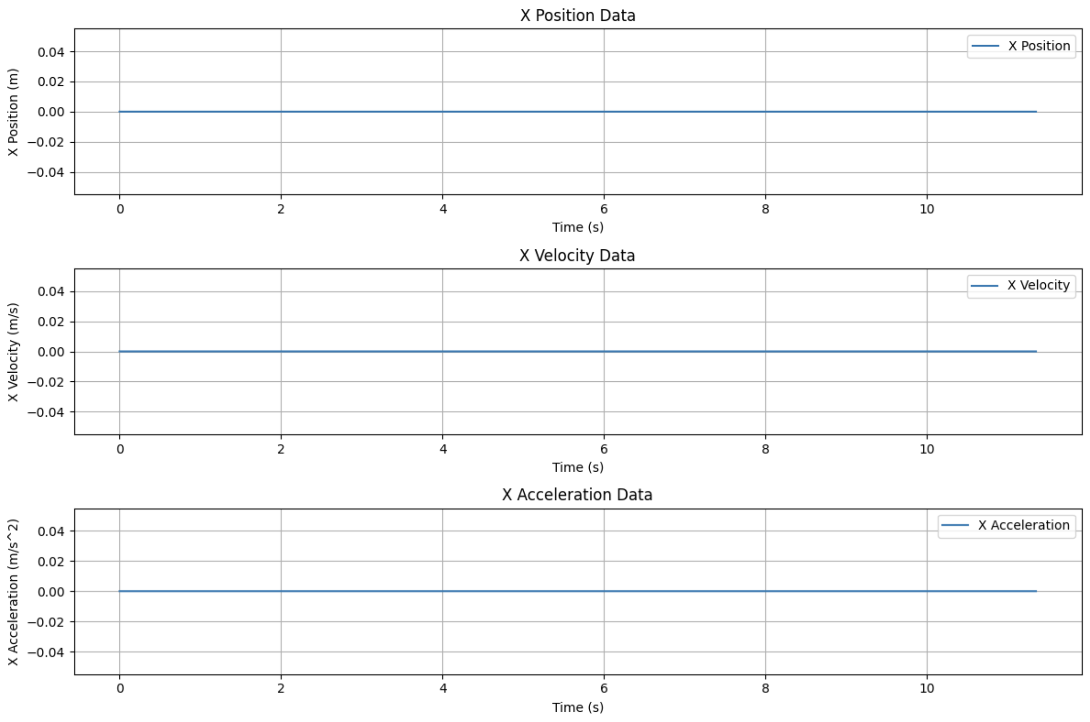
Recall when we were setting the parameters for the simulation, we set the gimbal_angle variable to $0rad$. This means the thruster won’t move at all and the rocket will shoot straight up and won’t move horizontally at all. That’s why the data in the X axis is all 0 because nothing is happening in the X axis yet.
Let’s try plotting out the trajectory of the rocket to get a better idea of how the rocket will fly:
# plot trajectory of rocket (2D)
plt.figure(figsize=(8, 5))

plt.plot(pos[:, 0], pos[:, 1], label='Rocket Trajectory', color='blue')
plt.scatter(pos[0, 0], pos[0, 1], color='green', label='Launch Point') # mark the launch point
plt.scatter(pos[-1, 0], pos[-1, 1], color='red', label='Impact Point') # mark the impact point
plt.axhline(0, color='black', linestyle='--', label='Ground') # ground level
plt.xlabel('X Position (m)')
plt.ylabel('Z Position (m)')
plt.title('Rocket Trajectory')
plt.legend()

plt.show()
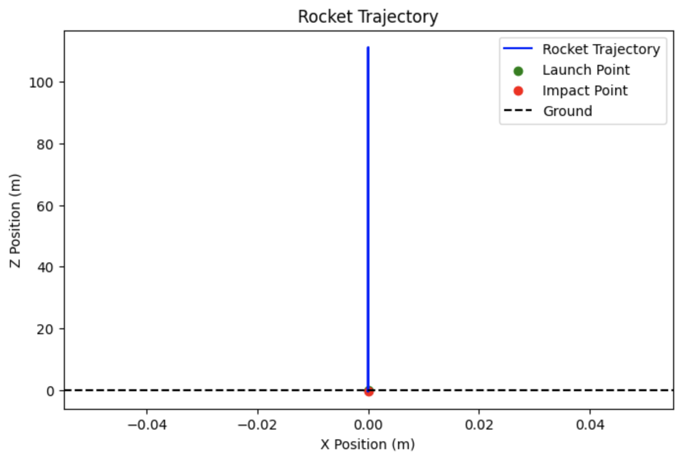
The rocket just shoots straight up to an altitude of around a little bit over $100m$ then drop straight down to the ground.
Plotting the simulation data with some gimbal angle
Now let’s see how our rocket will fly with some gimbal angle. To do this, we can just adjust our gimbal_angle variable. I’ll adjust it by a tiny bit:
gimbal_angle = -0.05 # radian
And let’s rerun the simulation.
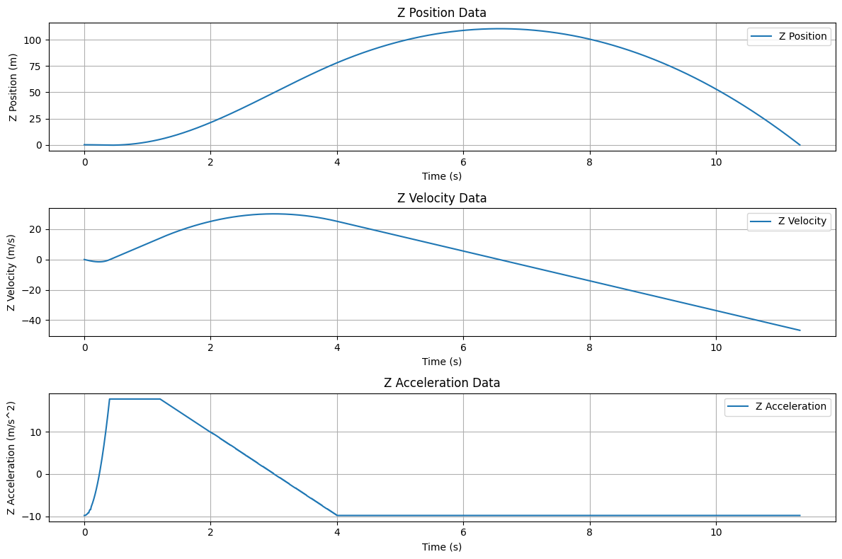
- Z axis data:
- X axis data:
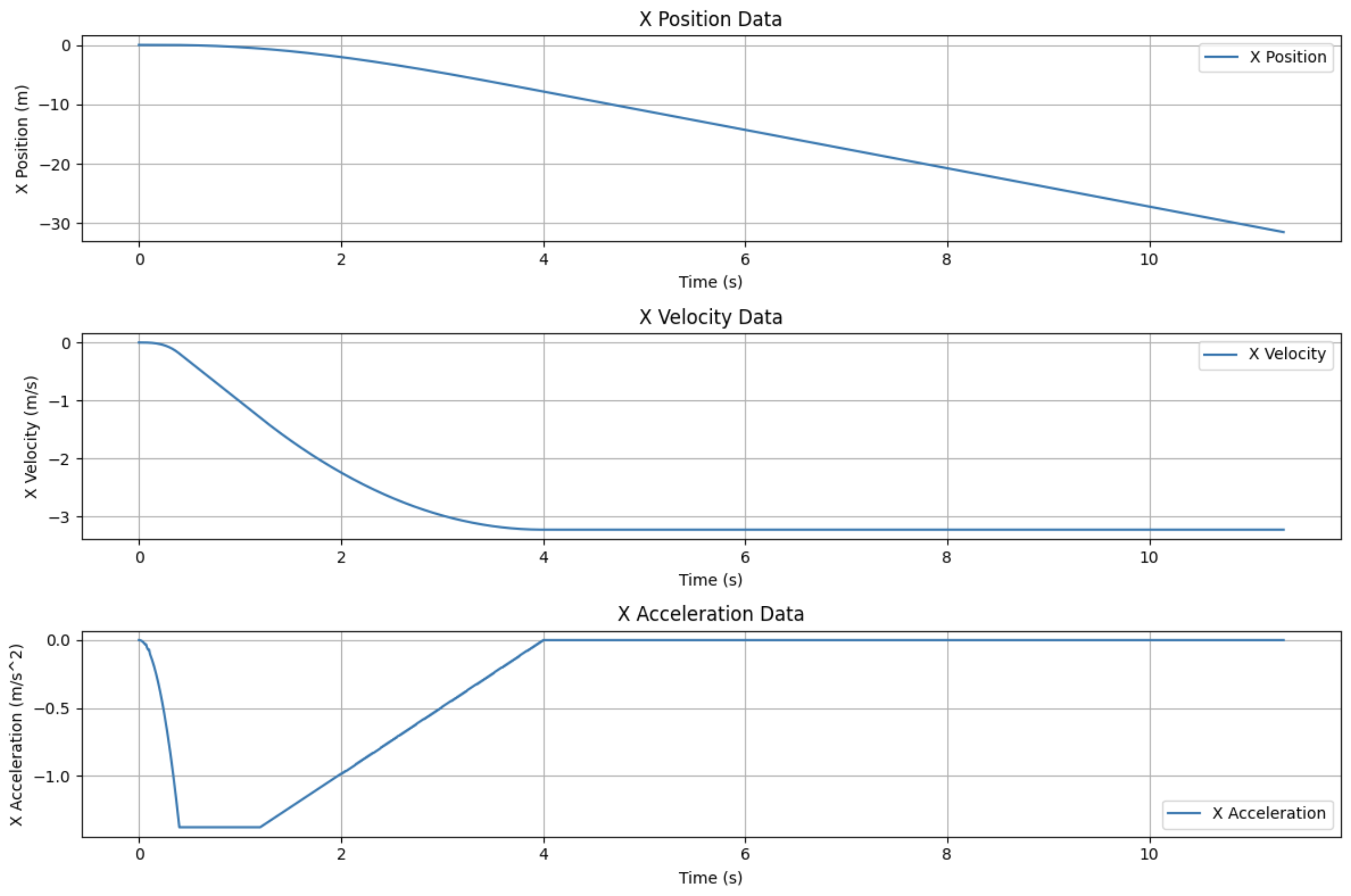
So the data on the Z axis remains unchanged from the last time we run the simulation, but the data on the X axis changed a lot. We can see that the X position data is gradually moving towards a different position, this indicates that the rocket is actually moving in the X axis. We can see the velocity data is also decreasing to the negative range since we’re moving to the left side. And we can also see the acceleration data on the X axis.
Let’s see the flight trajectory:
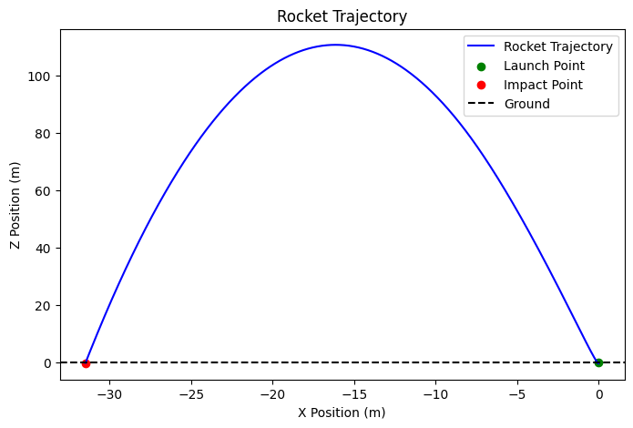
And there we go. The rocket flies all the way over $100m$ and land at just over $30m$ from its initial launch point. We have successfully modeled a TVC rocket in Python.
Conclusion
We have successfully modeled a TVC rocket in Python with 3 degrees of freedom. We’ve covered what 3 degrees of freedom is, what thrust curve is, how to implement some equations to model the rocket and how to plot out the simulated rocket’s data and trajectory.
There’s a lot more to be done for this project like more realistic thrust curve, add in other external factors such as wind and air resistances, and implement a PID or a thrust vector control method to control this rocket. I might get around implementing these things into the simulation in the future.
This was a very fun project. I definitely learned a lot about rocketry from this, and I hope you can learn more about rocketry and rocket dynamics simulation from this blog post.
You can check out the source code for this project here