The Lorenz System and The Butterfly Effect
If you’ve ever seen a movie about time travel, you’ll probably have heard of the term “The Butterfly Effect”. The Butterfly Effect got its name from a pretty interesting example: The flapping of a butterfly in the present can cause a hurricane in the future. It’s used extensively in time travel movies because if you somehow managed to time travel to the past and change the past, the future could be drastically altered from that small change due to how that small change compounded into bigger and bigger changes.
This pop culture implication is quite consistent with the real-world implication of chaos theory: For a given system, small changes in its initial condition could result in massive difference in the system’s evolution trajectory. These kinds of systems, which are highly sensitive to changes in the initial conditions, are chaotic.
I just want to be clear that chaotic systems are NOT random. Chaotic systems are deterministic. The evolution of these systems follow a unique pattern and is determined by their initial conditions. However, predictions of how the system will even in the long run is virtually impossible.
“Chaos: When the present determines the future, but the approximate present does not approximately determine the future” - Edward Lorenz
In order to get a closer look at chaos theory, we’ll explore one of the most infamous chaotic system: The Lorenz system, developed by Edward Lorenz, one of the pioneers in chaos theory.
Atmospheric convection
The Lorenz system was originally developed for modeling atmospheric convection, which is a process where heat and moisture is transported vertically through the atmosphere (Hot air goes up, cool air goes down). This rolling phenomenon occurs when the sun heats the air near Earth’s surface than air higher in the atmosphere or over bodies of water.
We can imagine a pot boiling some water. As the water at the bottom heats up, it expands and and becomes less dense, causing it to rise. The cooler, denser water at the top sinks to replace it, creating a continuous “rolling” cycle of motion known as convection. This convection motion is highly chaotic as fluid flows have the potential to exhibit chaotic behaviors. Thus, a mathematical model is required to fully understand this chaotic systems.
Edward Lorenz managed to derive a simple set of 3 ordinary differential equations that describes the atmospheric convection. These nonlinear equations describes the complex and unpredictable nature of the convection phenomenon.
The Lorenz equations
The Lorenz system is described by these 3 ordinary differential equations:
$$ \begin{aligned} \dot{x} &= \sigma (y - x) \\ \dot{y} &= x (\rho - z) - y \\ \dot{z} &= x y - \beta z \end{aligned} $$
We can think of the system in a 3 dimensional plane. $x$, $y$, $z$ each representing the system’s state its corresponding axis. $\sigma$, $\rho$, $\beta$ are system parameters that affect the evolution of the system. The output of the system is the instantaneous rate of change of the system in each axis. This derivative can then be used to update the system and describe how the system will continue evolving in time.
In the context of the atmospheric convection problem:
- $x$: Rate of convective motion in the fluid system
- $y$: Variation in horizontal temperature in the fluid layer
- $z$: Variation in vertical temperature in the fluid layer
- $\sigma$: Ratio of fluid viscosity to thermal conductivity (Prandtl number)
- $\rho$: The temperature difference driving the convection (Rayleigh number)
- $\beta$: Aspect ratio of the convection cells
These 3 equations are all ODEs, so we can solve them quite efficiently by using numerical methods like forward Euler, Runge-Kutta, etc.
Simulating the system
Let’s simulate the Lorenz system with Python.
Prerequisites: scipy, numpy, matplotlib.
import numpy as np
import matplotlib.pyplot as plt
from mpl_toolkits.mplot3d import Axes3D
from scipy import integrate
We’ll be using the odeint function from the scipy package in Python. This function allows us to solve ODEs efficiently. To use this function, we’ll first need to specify a time span that the system will be simulated over. I’ll set up a time span from 0 to 50 with a time step of 0.001, so the system will gradually go from time 0 to time 50 by stepping forward by 0.001 time.
dt = 0.001 # step
T = 50 # range
t = np.arange(0, T + dt, dt) # time span
Next, we’ll need to specify the starting condition of the system, which is the initial $x$, $y$, and $z$. We’ll also need to specify the parameters for the system $\sigma$, $\rho$, $\beta$. Lorenz used the values $10$, $28$, $8/3$ for each of the parameters respectively, which will make the system exhibit chaotic behaviors.
# initial condition
x0 = (0, 1, 20)

# parameters
sigma = 10
beta = 8 / 3
rho = 28
Now the function odeint needs to know what the ODEs of interest are. So let’s code up the 3 ODEs of the Lorenz system up in a function:
def lorenz(xyz, t0, sigma, beta, rho):
    x, y, z = xyz # current state

    x_dot = sigma * (y - x)
    y_dot = x * (rho - z) - y
    z_dot = x * y - beta * z

    return [x_dot, y_dot, z_dot]
With all the conditions and equations set up, we can now use odeint to simulate the system. I’ll use the relative tolerance (rtol) and absolute tolerance (atol) to limit error in the numerical integration. These tolerance values will ensure the error doesn’t exceed the tolerance value and making the solution more accurate. Once the odeint is finished simulating the system, we’ll get 3 vectors in return. The 3 vectors contain the values of $x$, $y$, and $z$ at each time step within the 0 to 50 time span.
# simulate system
x_t = integrate.odeint(lorenz, x0, t, (sigma, beta, rho), rtol=10**(-12), atol=10**(-12) * np.ones_like(x0))
x, y, z = x_t.T
Once the simulation is done, we can plot the result to visualize the solution:
fig = plt.figure()
ax = fig.add_subplot(projection='3d')

ax.plot(x, y, z, linewidth=1)
ax.scatter(x0[0], x0[1], x0[2], color='r')
ax.view_init(10, -50)

plt.show()
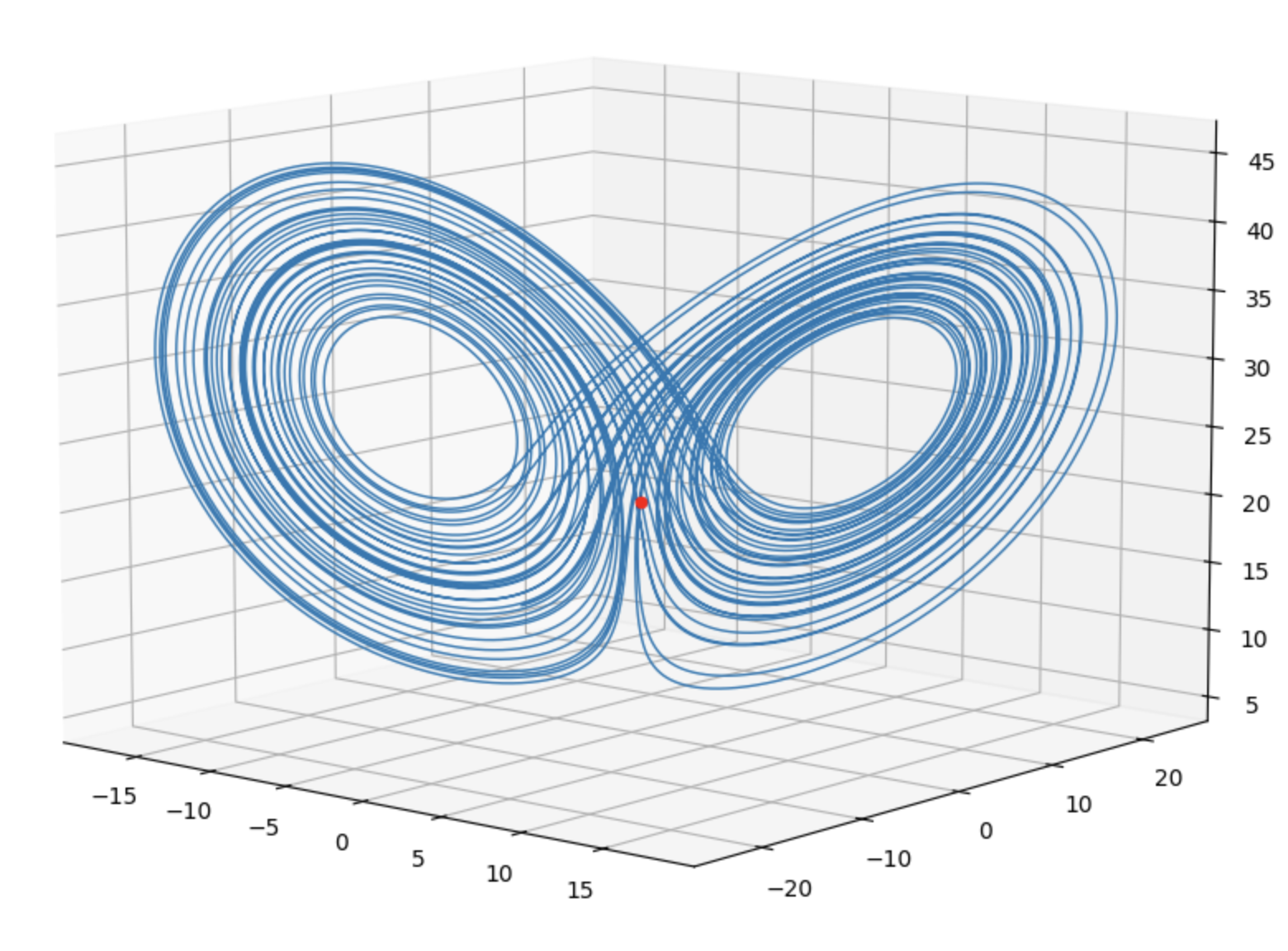
And the result is the beautiful chaotic behavior which kinda resembles the shape of a buttefly.

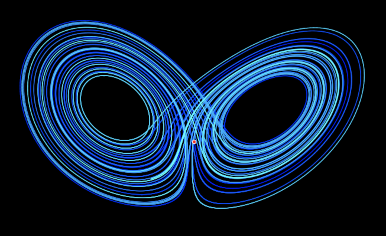
A fun thing we could do is plot the system with some color to make it look cooler. I’ll set the background to black, remove the axes and the grid, and set the color map of the plot to go from blue to cyan.
import matplotlib.colors as mcolors

fig = plt.figure()
ax = fig.add_subplot(projection='3d')

ax.set_facecolor("black")
fig.patch.set_facecolor("black")

cmap = mcolors.LinearSegmentedColormap.from_list("blue_cyan", ["blue", "cyan"])
colors = cmap(np.linspace(0, 1, len(x) - 1))

for i in range(len(x) - 1):
    ax.plot(x[i:i+2], y[i:i+2], z[i:i+2], color=colors[i], linewidth=1)
ax.scatter(x0[0], x0[1], x0[2], color='r', edgecolor='white')

ax.view_init(10, -50)
plt.axis('off')

plt.show()

Note how the system exhibit “rolling” behaviors, which is consistent with how atmostpheric convection works.
Conclusion
That was a glimpse into the world of chaos theory. The Lorenz system showed how a system’s behavior can vary drastically based on the initial condition. There are so many other dynamical systems, with many of them being chaotic. Chaos theory is a very exciting field and I hope this introduction will get you more excited and curious about this field.
Hope you enjoyed reading this blog post.